Regression model for recurrent event data

The regression model implemented in the reReg package accommodate informative censoring via the use of a subject-specific frailty variable. In contrast to existing frailty models, the implemented estimation procedure does not require distributional information on the frailty variable. Using the borrowing-strength approach in the estimating procedure, our model allows users to specify any combination of the sub-models between the recurrent event process and the terminal events when they are fitted jointly.

In this vignette, we demonstrate how to use the reReg() function in the reReg package to fit semiparametric regression models to recurrent event data.

Notations

Let \(N(t)\) be the number of recurrent events occurring over the interval \([0, t]\) and \(D\) be the failure time of interest subjects to right censoring by \(C\). Define the composite censoring time \(Y = \min(D, C, \tau)\) and the failure event indicator \(\Delta = I\{D\le \min(C, \tau)\}\), where \(\tau\) is the maximum follow-up time. We assume the recurrent event process \(N(\cdot)\) is observed up to \(Y\). Let \(X\) be a \(p\)-dimensional covariate vector. Consider a random sample of \(n\) subjects, the observed data are independent and identically distributed (iid) copies of \(\{Y_i, \Delta_i, X_i, N_i(t), 0\le t\le Y_i\}\), where the subscript \(i\) denotes the index of a subject for \(i= 1, \ldots, n\). Let \(m_i = N_i(Y_i)\) be the number of recurrent events the \(i\)th subject experienced before time \(Y_i\), then the jump times of \(N_i(t)\) give the observed recurrent event times \(t_{i1}, \ldots, t_{im_i}\) when \(m_i > 0\). Thus, the observed data can also be expressed as iid copies of \(\{Y_i, \Delta_i, X_i, m_i, (t_{i1}, \ldots, t_{m_i})\}\). The primary interests in recurrent event data analysis is in making inference about the recurrent event process and the failure event and understanding the corresponding covariate effects.

Model assumption

We assume a generalized joint frailty scale-change model for the rate function of the recurrent event process and the hazard function of the failure time formulated as follow: \[\begin{equation} \begin{cases} \lambda(t) = \displaystyle Z\lambda_0(te^{X^\top\alpha})e^{X^\top\beta},&\\ h(t) = \displaystyle Zh_0(te^{X^\top\eta})e^{X^\top\theta}, &t\in[0, \tau], \end{cases} \end{equation}\] where \(Z\) is a latent shared frailty variable to account for association between the two types of outcomes, \(\lambda_0(\cdot)\) is the baseline rate function, \(h_0(\cdot)\) is the baseline hazard function, and the regression coefficients \((\alpha, \eta)\) and \((\beta, \theta)\) correspond to the shape and size parameters of the rate function and hazard function, respectively. In contrast to many shared-frailty models that require a parametric assumption, following the idea of Wang, Qin, and Chiang (2001), the reReg() function implements semiparametric estimation procedures that do not require the knowledge about the frailty distribution. As a result, the dependence between recurrent events and failure event is left unspecified and the proposed implementations accommodate informative censoring. The reReg() function fits the recurrent event data under the above joint model setting. The arguments of reReg() are as follows

> library(reReg)
> args(reReg)

function (formula, data, subset, model = "cox", B = 0, se = c("boot", 
    "sand"), control = list()) 
NULL

formula a formula object, with the response on the left of a “~” operator, and the predictors on the right. The response must be a recurrent event survival object as returned by function Recur. See the vignette on Visualization of recurrent event data or Introduction to formula response function Recur() for examples in creating Recur objects.
data an optional data frame in which to interpret the variables occurring in the formula.
B a numeric value specifies the number of bootstrap (or resampling) for variance estimation. When B = 0, variance estimation will not be performed.
model a character string specifying the underlying model.
se a character string specifying the method for standard error estimation.
control a list of control parameters.

Specifying model via the `model` argument

When the interest is the covariate effects on the risk of recurrent events and the terminal event is treated as nuisances, model = "cox" and model = "gsc" give the Cox-type model and the generalized scale-change rate model considered in Wang, Qin, and Chiang (2001) and Xu et al. (2020), respectively. When the recurrent event process and the terminal events are modeled jointly, the types of rate function and hazard function can be specified simultaneously in model separated by ``|’’. The model types for the hazard function are cox, ar, am, and gsc. For examples, the joint frailty Cox-type model of Huang and Wang (2004) and the joint frailty accelerated mean model of Xu et al. (2017) can be called by model = "cox|cox" and model = "am|am", respectively. Depending on the application, users can specify different model types for the rate function and the hazard function. For example, model = "cox|ar" postulate a Cox-type proportional model for the recurrent event rate function and an accelerated rate model for the terminal event hazard function, or \(\alpha = \theta = 0\) in (1).

Variance estimation

The nonparametric bootstrap method for clustered data is adopted to estimate the standard errors of the estimators. The bootstrap samples are formed by resampling the subjects with replacement of the same size from the original data. The above estimating procedures are then applied to each bootstrap sample to provide one draw of the bootstrap estimate. With a large number of replicates, the asymptotic variance matrices are estimated by the sample variance of the bootstrap estimates. In an attempt to overcome the computational burden in bootstrap variance estimation, parallel computing techniques based on methods in the parallel package will be applied when boot.parallel = TRUE}. The number of CPU cores used in the parallel computing is controlled by the argument boot.parCl}, whose default value is half of the total number of CPU cores available on the current host identified by parallel::detectCores() \%/\% 2}. When fitting the generalized scale-change rate model of Xu et al. (2020), e.g., with model = "sc", an efficient resampling-based sandwich estimator is also available via se = "sand". The number of bootstrap or resampling is controlled by the argument B. When B = 0 (default), the variance estimation procedure will not be performed and only the point estimates will be returned, which can be useful when the variance estimation is time consuming. Future work will be devoted to generalize the efficient resampling-based sandwich estimator to all the sub-models.

The `control` list

The complete control list consists of the following parameters:

eqType is a character string used to specify whether the log-rank-type ("logrank") or the Gehan-type ("gehan") estimating equation is used in the estimating procedure.
solver is a character string used to specify the equation solver used for root search; the available options are BBsolve, dfsane, BBoptim, and optim (the first three options loads the corresponding equation solver from package BB (Varadhan and Gilbert 2009)).
tol is a numerical value used to specify the absolute error tolerance in solving the estimating equations. The default value is \(10^{-7}\).
ini is a list of initial values used in the root-finding algorithms. The list members alpha, beta, eta, and theta correspond to the parameters \(\alpha\), \(\beta\), \(\eta\), and \(\theta\) in Model~, respectively. The default values for these initial values are zeros.
boot.parallel is an logical value indicating whether parallel computation will be applied when se = "boot" is called.
boot.parCl is an integer value specifying the number of CPU cores to be used when parallel = TRUE. The default value is half the CPU cores on the current host.

The default equation solver ("BB::dfsane") uses the derivative-free Barzilai-Borwein spectral approach for solving nonlinear equations implemented in dfsane() from the package BB (Varadhan and Gilbert 2009). Setting solver = "BB::BBsolve" calls the wrapper function BBsolve() in the BB package to locate a root with different Barzilai-Borwein step-lengths, non-monotonicity parameters, and initialization approaches. Based on our observation, the "BB::BBsolve" algorithm generally exhibited more reliable convergence but the solver = "BB::dfsane" algorithm provides a better balance between convergence and speed. The alternative options, solver = "BB::BBoptim" and solver = "optim", attempts to identify roots by minimizing the \(\ell_2\)-norm of the estimating functions. The options solver = "BB::BBoptim" and solver = "optim" call the BBoptim() function from the package BB and the base function optim(), respectively.

Examples

We will illustrate the usage of reReg with simulated data generated from the simGSC() function. Readers are referred to the vignette on Simulating recurrent event data for using simGSC() to generate recurrent event data.

Joint Cox model of Huang and Wang (2004)

A simulated data following the joint Cox model can be generated by

> set.seed(1); datCox <- simGSC(200, summary = TRUE)

Call: 
simGSC(n = 200, summary = TRUE)

Summary:
Sample size:                                    200 
Number of recurrent event observed:             710 
Average number of recurrent event per subject:  3.55 
Proportion of subjects with a terminal event:   0.585 
Median time-to-terminal event:                  10.078

Since the default parameters in simGSC() are \(\alpha = (0, 0)^\top\), \(\beta = (-1, -1)^\top\), \(\eta = (0, 0)^\top\), and \(\theta = (-1, -1)^\top\), the underlying true model has the form: \[\begin{cases} \lambda(t) = Z \lambda_0(t)e^{-X_1 - X_2}, &\\ h(t) = Z h_0(t)e^{-X_1 - X_2}, & t\in[0, 60]. \end{cases}\] The model fit is

> fit.cox <- reReg(Recur(t.start %to% t.stop, id, event, status) ~ x1 + x2, 
+                  B = 200, data = datCox, model = "cox|cox")
> summary(fit.cox)

Call: 
reReg(formula = Recur(t.start %to% t.stop, id, event, status) ~ 
    x1 + x2, data = datCox, model = "cox|cox", B = 200)

Recurrent event process:
   Estimate   StdErr z.value   p.value    
x1 -0.99760  0.15371 -6.4902 8.570e-11 ***
x2 -1.08084  0.14564 -7.4215 1.158e-13 ***

Terminal event:
   Estimate  StdErr z.value   p.value    
x1  1.29806 0.28137  4.6134 3.962e-06 ***
x2  1.33244 0.32677  4.0777 4.549e-05 ***

The baseline functions can be plotted via plot():

> plot(fit.cox)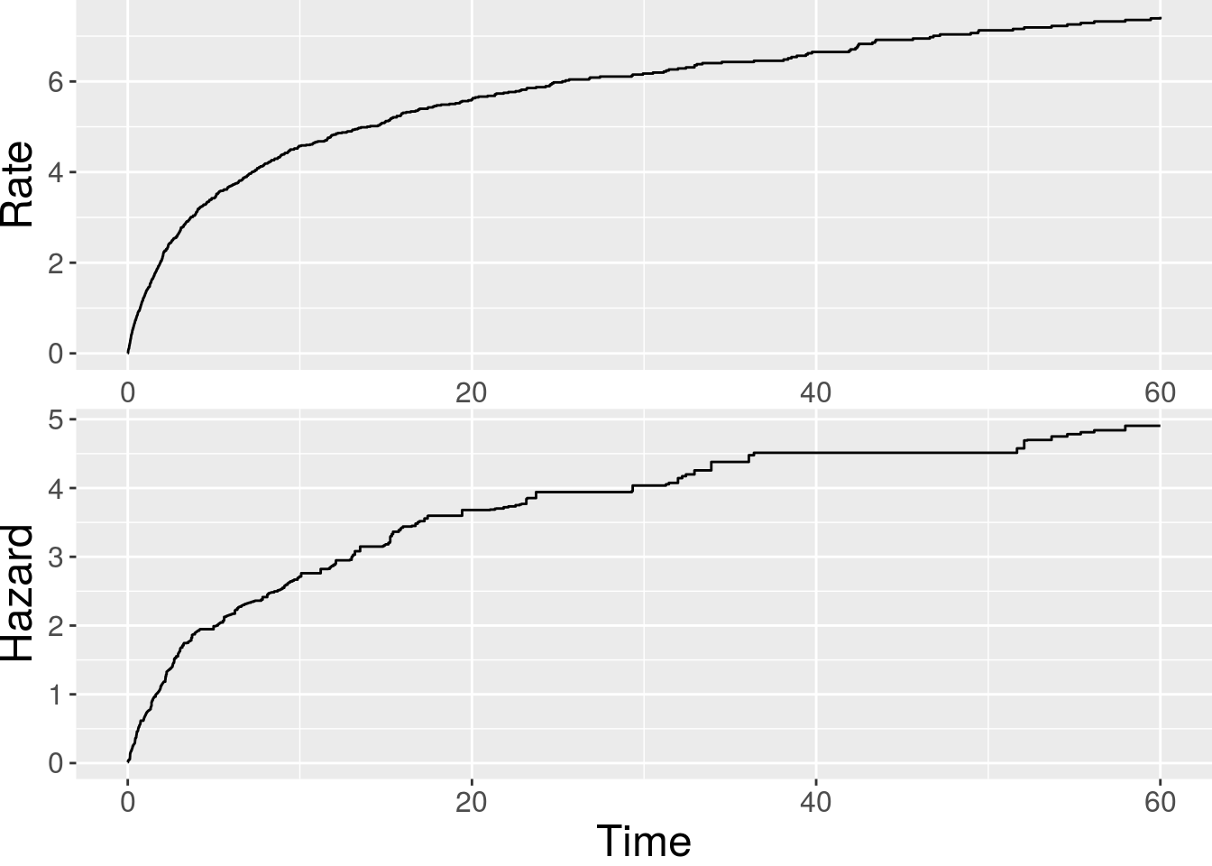

Joint accelerated mean model of Xu et al. (2017)

A simulated data following the joint accelerated mean model can be generated by

> set.seed(1)
> par0 <- list(alpha = c(1, 1), beta = c(1, 1), eta = -c(1, 1), theta = -c(1, 1))
> datam <- simGSC(200, par = par0, summary = TRUE)

Call: 
simGSC(n = 200, summary = TRUE, para = par0)

Summary:
Sample size:                                    200 
Number of recurrent event observed:             1122 
Average number of recurrent event per subject:  5.61 
Proportion of subjects with a terminal event:   0.4

The underlying true model has the form: \[\begin{cases} \lambda(t) = Z \lambda_0(te^{X_1 + X_2})e^{X_1 + X_2}, &\\ h(t) = Z h_0(te^{-X_1 - X_2})e^{-X_1 - X_2}, & t\in[0, 60]. \end{cases}\] The model fit is

> fit.am <- reReg(Recur(t.start %to% t.stop, id, event, status) ~ x1 + x2,
+                 B = 200, data = datam, model = "am|am")
> summary(fit.am)

Call: 
reReg(formula = Recur(t.start %to% t.stop, id, event, status) ~ 
    x1 + x2, data = datam, model = "am|am", B = 200)

Recurrent event process:
   Estimate  StdErr z.value   p.value    
x1  0.75204 0.25470  2.9527   0.00315 ** 
x2  1.10920 0.27356  4.0547 5.019e-05 ***

Terminal event:
   Estimate   StdErr z.value  p.value   
x1 -1.74571  0.56071 -3.1134 0.001849 **
x2 -1.18901  0.57962 -2.0514 0.040231 *

The baseline functions can be plotted via plot():

> plot(fit.am)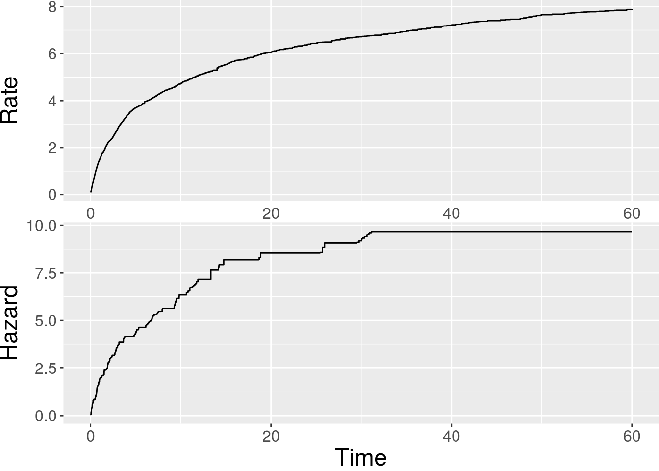

Joint Cox/accelerated rate model

A simulated model following a special case of the generalized scale-change model where the rate function has a Cox structure and the hazard function has an accelerated rate model structure can be generated by

> set.seed(1)
> par0 <- list(eta = c(1, 1), theta = c(0, 0))
> datCoxAr <- simGSC(200, par = par0, summary = TRUE)

Call: 
simGSC(n = 200, summary = TRUE, para = par0)

Summary:
Sample size:                                    200 
Number of recurrent event observed:             678 
Average number of recurrent event per subject:  3.39 
Proportion of subjects with a terminal event:   0.34

The underlying true model has the form: \[\begin{cases} \lambda(t) = Z \lambda_0(t)e^{-X_1 - X_2}.&\\ h(t) = Z h_0(te^{X_1 + X_2})& t\in[0, 60]. \end{cases}\] The model fit is

> fit.CoxAr <- reReg(Recur(t.start %to% t.stop, id, event, status) ~ x1 + x2,
+                    B = 200, data = datCoxAr, model = "cox|ar")
> summary(fit.CoxAr)

Call: 
reReg(formula = Recur(t.start %to% t.stop, id, event, status) ~ 
    x1 + x2, data = datCoxAr, model = "cox|ar", B = 200)

Recurrent event process:
   Estimate   StdErr z.value   p.value    
x1 -0.94955  0.15750 -6.0289 1.651e-09 ***
x2 -0.88239  0.16338 -5.4010 6.627e-08 ***

Terminal event:
   Estimate  StdErr z.value p.value  
x1  1.40308 0.56318  2.4913 0.01273 *
x2  1.06758 0.58527  1.8241 0.06814 .

The baseline functions can be plotted via plot():

> plot(fit.CoxAr)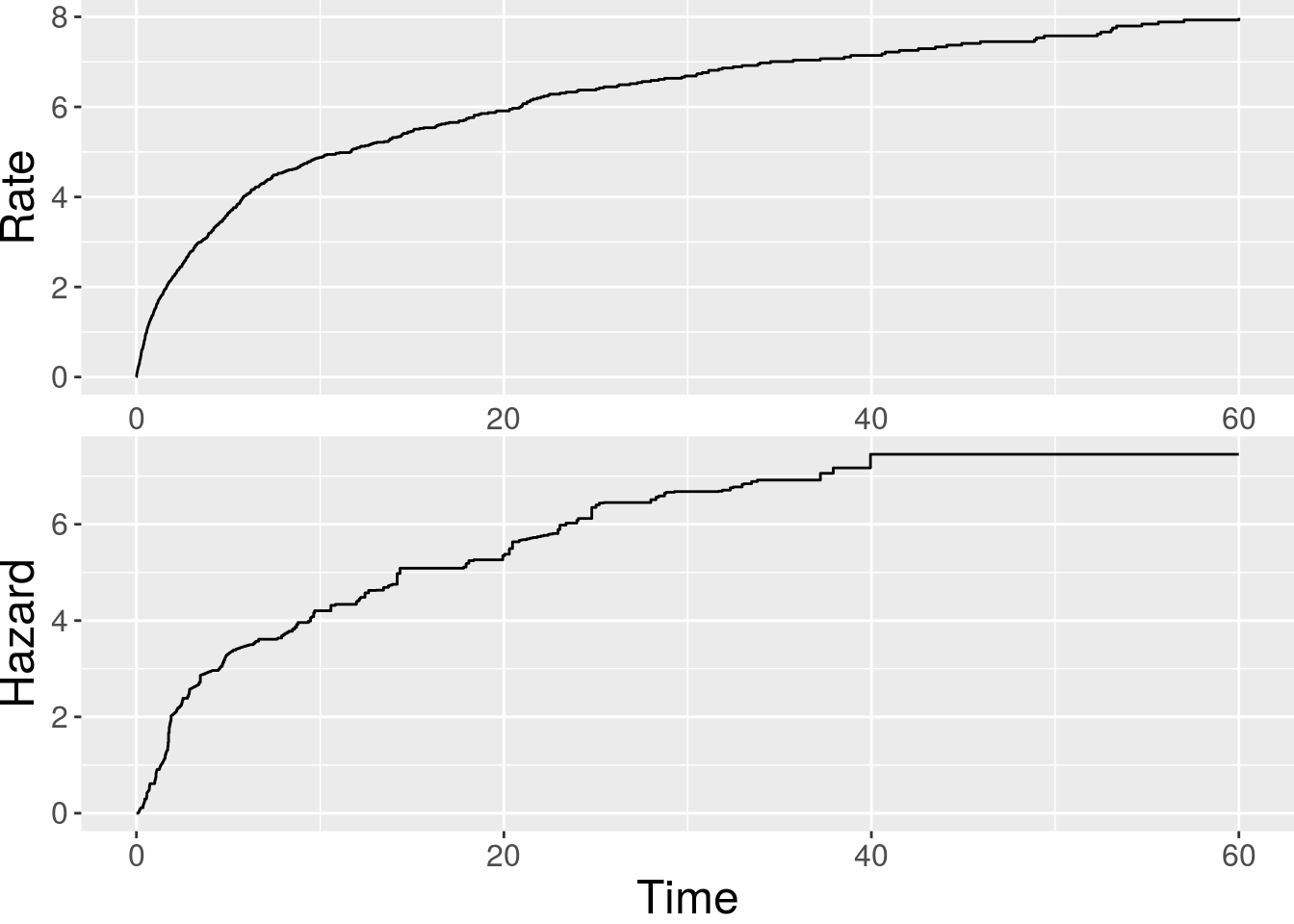

Other popular methods

Some methods that assumes Z = 1 and requires independent censoring are also implemented in reReg. These includes the methods proposed by Lin et al. (2000), Ghosh and Lin (2002), and Ghosh and Lin (2003), that can be called by specifying model = "cox.LWYY", model = "cox.GL", and model = "am.GL", respectively.

It is also worth noting that methods in multi-state models could also be applied to analyze recurrent events data. See the vignette on Multi-state models and competing risks for more details.

Reference

Ghosh, Debashis, and D. Y. Lin. 2002. “Marginal Regression Models for Recurrent and Terminal Events.” Statistica Sinica 12 (3): 663–88.

———. 2003. “Semiparametric Analysis of Recurrent Events Data in the Presence of Dependent Censoring.” Biometrics 59 (4): 877–85.

Huang, Chiung-Yu, and Mei-Cheng Wang. 2004. “Joint Modeling and Estimation for Recurrent Event Processes and Failure Time Data.” Journal of the American Statistical Association 99 (468): 1153–65.

Lin, D. Y., L. J. Wei, I. Yang, and Z. Ying. 2000. “Semiparametric Regression for the Mean and Rate Functions of Recurrent Events.” Journal of the Royal Statistical Society: Series B 62 (4): 711–30.

Varadhan, Ravi, and Paul Gilbert. 2009. “BB: An R Package for Solving a Large System of Nonlinear Equations and for Optimizing a High-Dimensional Nonlinear Objective Function.” Journal of Statistical Software 32 (4): 1–26. http://www.jstatsoft.org/v32/i04/.

Wang, Mei-Cheng, Jing Qin, and Chin-Tsang Chiang. 2001. “Analyzing Recurrent Event Data with Informative Censoring.” Journal of the American Statistical Association 96 (455): 1057–65.

Xu, Gongjun, Sy Han Chiou, Chiung-Yu Huang, Mei-Cheng Wang, and Jun Yan. 2017. “Joint Scale-Change Models for Recurrent Events and Failure Time.” Journal of the American Statistical Association 112 (518): 794–805.

Xu, Gongjun, Sy Han Chiou, Jun Yan, Kieren Marr, and Chiung-Yu Huang. 2020. “Generalized Scale-Change Models for Recurrent Event Processes Under Informative Censoring.” Statistica Sinica 30: 1773–95.

Sy Han (Steven) Chiou

2024-05-20

Notations

Model assumption

Specifying model via the `model` argument

Variance estimation

The `control` list

Examples

Joint Cox model of Huang and Wang (2004)

Joint accelerated mean model of Xu et al. (2017)

Joint Cox/accelerated rate model

Other popular methods

Reference

Regression model for recurrent event data

Sy Han (Steven) Chiou

2024-05-20

Notations

Model assumption

Specifying model via the model argument

Variance estimation

The control list

Examples

Joint Cox model of Huang and Wang (2004)

Joint accelerated mean model of Xu et al. (2017)

Joint Cox/accelerated rate model

Other popular methods

Reference

Specifying model via the `model` argument

The `control` list