Introduction to censCov
Sy Han (Steven) Chiou
2019-05-21
Source:vignettes/censCov-examples.Rmd
censCov-examples.RmdIn this vignette, we demonstrate how to use the thlm function in censCov package to fit linear regression model with censored covariate using the methods proposed in Qian et al. (2018).
Notations
Suppose the linear regression model: \[ Y = \alpha_0 + \alpha_1X + \boldsymbol{\alpha}_2^\top \bf Z + \epsilon, \] where \(Y\) is the response variable, \(X\) is the covariate of interest which is subject to right censoring, \(\bf Z\) is a \(p\times 1\) vector of additional covariates that are completely observed, \(\epsilon\) is the random error term with mean 0 and finite variance, and the \(\alpha\)’s are the corresponding regression coefficients. We assume \(epsilon\) is independent of \(X\), \(\bf Z\), and \(C\), where \(C\) is the right censoring that potentially censors \(X\). The primary scientific interest is in the parameter \(\alpha_1\), which captures the association between \(Y\) and \(X\). The thlm function provides
- a test for \(H_o: \alpha_1 = 0\) against its complement;
- unbiased estimation of the regression coefficient of the censored covariate.
The thlm function
The thlm function presents the threshold regression approaches for linear regression models with a covariate that is subject to random censoring. The threshold regression methods allow for immediate testing of the significance of the effect of a censored covariate. The censCov package can be installed from CRAN with
> install.packages("censCov")or from GitHub with
> devtools::install_github("stc04003/censCov")The arguments of the thlm function are as follows:
function (formula, data, method = c("cc", "reverse", "deletion-threshold",
    "complete-threshold", "all"), B = 0, subset, x.upplim = NULL,
    t0 = NULL, control = thlm.control())
NULL-
formulais a formula expression in the form ofresponse ~ predictors. The response variable is assumed to be fully observed. Thethlmfunction can accommodate at most one censored covariate, which is entered in the formula as anSurvobject; seesurvival::Survfor more detail. If all the covariates are uncensored, thethlmfunction returns almobject. -
datais an optional data frame, list or environment contains variables in theformulaand thesubsetargument. If this is left unspecified, the variables are taken from the environment from whichthlmis called. -
methodis a character string specifying the threshold regression methods to be used. The following are permitted:-
ccfor complete-cases regression -
reversefor complete-cases regression -
deletion-thresholdfor complete-cases regression -
complete-thresholdfor complete-cases regression -
allfor complete-cases regression
-
-
Bis a numeric value specifies the bootstrap size for estimating the standard error of the regression coefficient for the censored covariate whenmethod = "deletion-threshold"ormethod = "complete-threshold". WhenB = 0(default), only the beta estimate will be displayed. -
subsetis an optional vector specifying a subset of observations to be used in the fitting process. -
x.upplimis an optional number value specifies the upper support of the censored covariate. When left unspecified, the maximum of the censored covariate will be used. -
t0is an optional numeric value specifies the threshold whenmethod = "deletion-threshold"ormethod = "complete-threshold". When left unspecified, an optimal threshold will be determined to optimize test power. -
controlis a list of threshold parameters including:-
t0.intervalcontrols the end points of the interval to be searched for the optimal threshold whent0is left unspecified -
t0.plotcontrols whether the objective function will be plotted. When t0.plot is true, both the rawt0.plotvalues and the smoothed estimates (using local polynomial regression fitting) are plotted.
-
Illustrative (simulated) data
We will illustrate the usage of thlm with a simulated data that is generated as below:
> simDat <- function(n) {
+   X <- rexp(n, 3)
+   Z <- runif(n, 1, 6)
+   Y <- 0.5 + 0.5 * X - 0.5 * Z + rnorm(n, 0, .75)
+   cstime <- rexp(n, .75)
+   delta <- (X <= cstime) * 1
+   X <- pmin(X, cstime)
+   data.frame(Y = Y, X = X, Z = Z, delta = delta)
+ }
> set.seed(1)
> head(dat <- simDat(200), 10)
Y X Z delta
1 -1.4004305 0.25172728 5.432294 1
2 -0.6842887 0.39388093 3.359654 1
3 -0.5541144 0.04856891 1.545505 1
4 0.1832982 0.04659842 2.666390 1
5 -2.5467871 0.14535621 5.187083 1
6 -0.6450906 0.49887130 2.384249 0
7 -2.0134650 0.40985402 3.935176 1
8 -2.5030175 0.17989428 5.183661 1
9 0.6904316 0.31885583 1.355770 1
10 -1.4071626 0.04901533 4.513894 1The columns in the simulated data set, dat, are
-
Yis the response variable -
Xis the covariate of interest whendelta = 1or the right censored value whendelta = 0 -
Zis an additional covariate that is completely observed -
deltais the censoring indicator forX
The average censoring percentage is about 20%.
Methods
The following methods for censored covariates are implemented in thlm.
Complete cases
When method = "cc", thlm removes rows with delta = 0 and fits the linear model via lm.
> thlm(Y ~ Surv(X, delta) + Z, data = dat, method = "cc")
 Call: thlm(formula = Y ~ Surv(X, delta) + Z, data = dat, method = "cc")

 Hypothesis test of association
H0: a1 = 0, p-value = 0.1028
or
> thlm(Y ~ X + Z, data = dat, subset = delta == 1)
 Call: thlm(formula = Y ~ X + Z, data = dat, subset = delta == 1)

 Hypothesis test of association
 H0: a1 = 0, p-value = 0.1047
The two \(p\)-values differs a bit because the thlm returns the Wald \(p\)-value.
Reverse survival regression
Call:
thlm(formula = Y ~ Surv(X, delta) + Z, data = dat, method = "rev")

 Reverse survival regression

 Coefficients:
  Estimate   StdErr z.value p.value
Y -0.18333  0.10056  -1.823  0.0683 .
---
Signif. codes:  0 '***' 0.001 '**' 0.01 '*' 0.05 '.' 0.1 ' ' 1
Deletion threshold regression
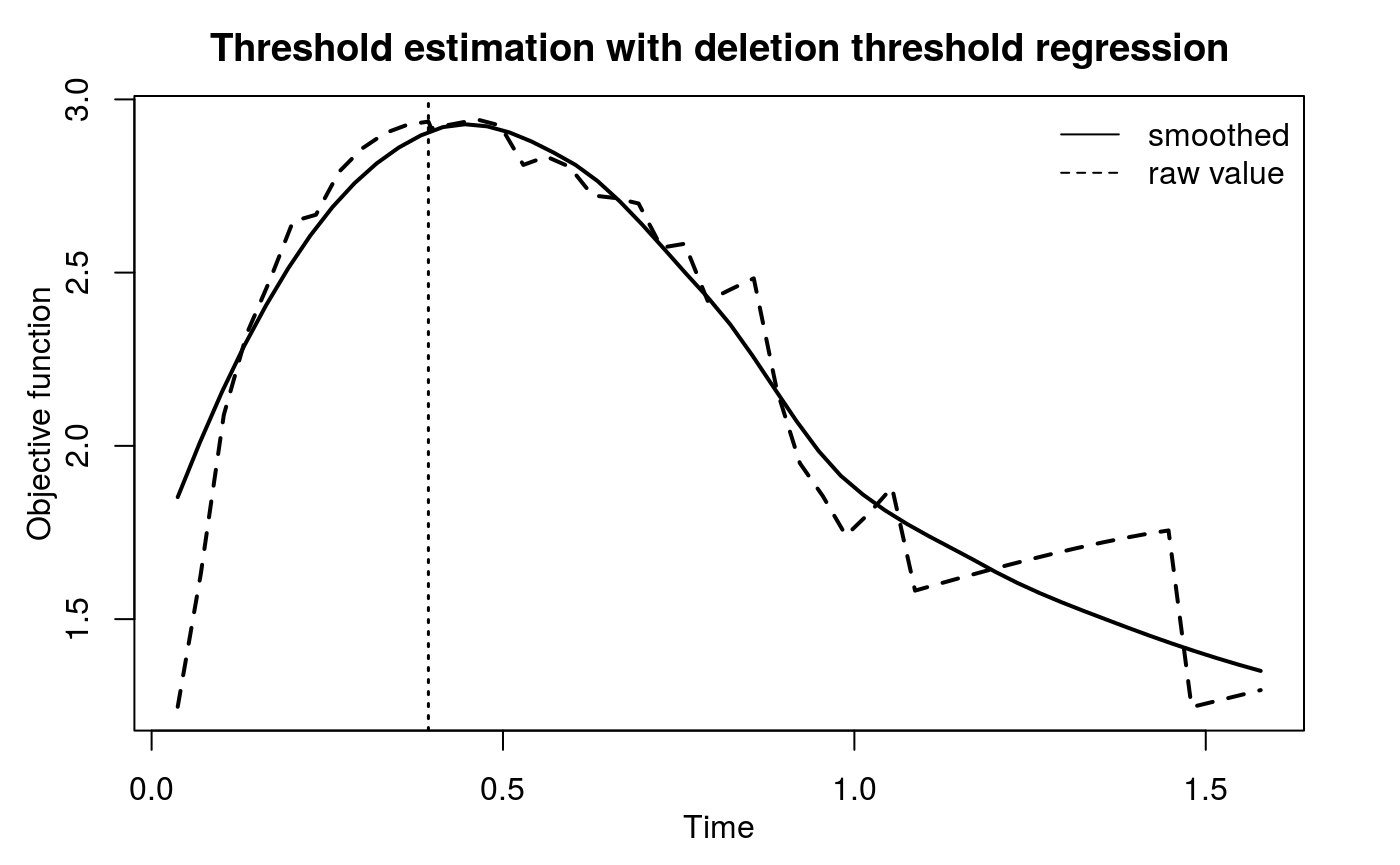
Call:
thlm(formula = Y ~ Surv(X, delta) + Z, data = dat, method = "del",
    B = 100)

 Deletion threshold regression
 Optimal threshold is 0.394

 Coefficients:
      Estimate    StdErr  z.value   p.value
a1:X  0.642742  0.235796   2.7258  0.006414 **
a2:Z -0.527387  0.039061 -13.5018 < 2.2e-16 ***
b1:X  0.307045  0.117716   2.6084  0.009098 **
---
Signif. codes:  0 '***' 0.001 '**' 0.01 '*' 0.05 '.' 0.1 ' ' 1

Under the assumption that X is independent of Z given X*. See ?thlm for more detail.
Complete threshold regression
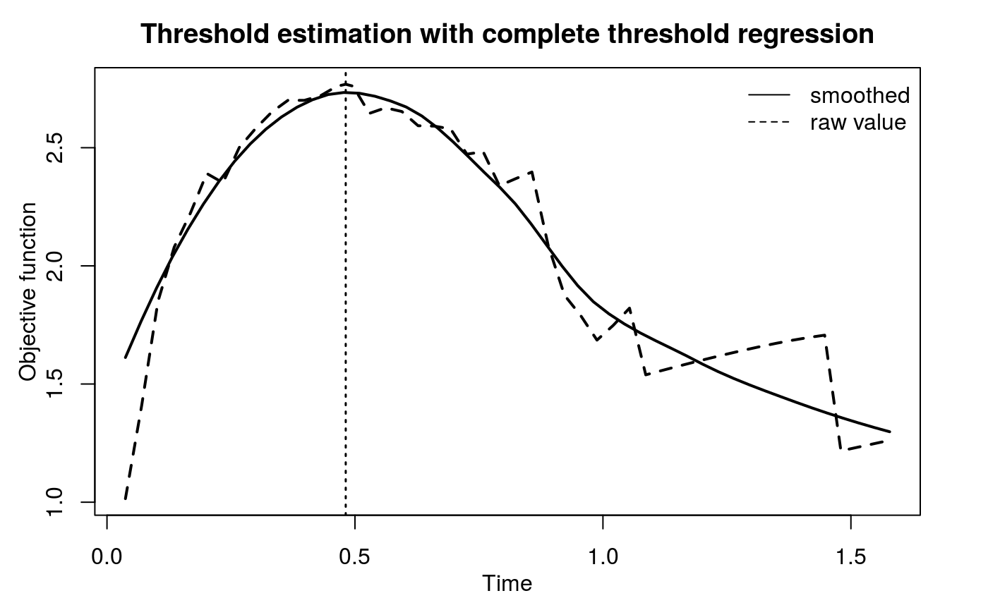
Call:
thlm(formula = Y ~ Surv(X, delta) + Z, data = dat, method = "com",
    B = 100)

 Complete threshold regression
 Optimal threshold is 0.481

 Coefficients:
      Estimate    StdErr  z.value p.value
a1:X  0.368099  0.304016   1.2108  0.2260
a2:Z -0.521533  0.036569 -14.2617  <2e-16 ***
b1:X  0.185574  0.138638   1.3386  0.1807
---
Signif. codes:  0 '***' 0.001 '**' 0.01 '*' 0.05 '.' 0.1 ' ' 1

Under the assumption that X is independent of Z given X*. See ?thlm for more detail.
All
The thlm function allows method = "all" that runs the complete cases analysis, reverse survival regression, deletion threshold regression, and complete threshold regression at once.
> summary(thlm(Y ~ Surv(X, delta) + Z, data = dat, method = "all", B = 100,
+              control = list(t0.plot = FALSE)))
Call:
thlm(formula = Y ~ Surv(X, delta) + Z, data = dat, method = "all",
B = 100, control = list(t0.plot = FALSE))
Complete-case regression
Coefficients:
Estimate StdErr z.value p.value
X 0.345912 0.212040 1.6314 0.1028
Z -0.526268 0.040216 -13.0861 <2e-16 ***
---
Signif. codes: 0 '***' 0.001 '**' 0.01 '*' 0.05 '.' 0.1 ' ' 1
Reverse survival regression
Coefficients:
Estimate StdErr z.value p.value
Y -0.18333 0.10056 -1.823 0.0683 .
---
Signif. codes: 0 '***' 0.001 '**' 0.01 '*' 0.05 '.' 0.1 ' ' 1
Deletion threshold regression
Optimal threshold is 0.394
Coefficients:
Estimate StdErr z.value p.value
a1:X 0.642742 0.264088 2.4338 0.014941 *
a2:Z -0.527387 0.039061 -13.5018 < 2.2e-16 ***
b1:X 0.307045 0.117716 2.6084 0.009098 **
---
Signif. codes: 0 '***' 0.001 '**' 0.01 '*' 0.05 '.' 0.1 ' ' 1
Complete threshold regression
Optimal threshold is 0.481
Coefficients:
Estimate StdErr z.value p.value
a1:X 0.368099 0.308850 1.1918 0.2333
a2:Z -0.521533 0.036569 -14.2617 <2e-16 ***
b1:X 0.185574 0.138638 1.3386 0.1807
---
Signif. codes: 0 '***' 0.001 '**' 0.01 '*' 0.05 '.' 0.1 ' ' 1
Under the assumption that X is independent of Z given X*. See ?thlm for more detail.FAQ
Can thlm fit model with one censored covariate (\(X\)) without any fully observed covaraite (\(Z\))?
Yes. For example:
> summary(thlm(Y ~ Surv(X, delta), data = dat, method = "all", B = 100,
+              control = list(t0.plot = FALSE)))
Call:
thlm(formula = Y ~ Surv(X, delta), data = dat, method = "all",
B = 100, control = list(t0.plot = FALSE))
Complete-case regression
Coefficients:
Estimate StdErr z.value p.value
X 0.10360 0.30109 0.3441 0.7308
Reverse survival regression
Coefficients:
Estimate StdErr z.value p.value
Y -0.059851 0.076203 -0.7854 0.4322
Deletion threshold regression
Optimal threshold is 0.394
Coefficients:
Estimate StdErr z.value p.value
a1:X 0.49723 0.34765 1.4303 0.1526
b1:X 0.23753 0.16906 1.4051 0.1600
Complete threshold regression
Optimal threshold is 0.481
Coefficients:
Estimate StdErr z.value p.value
a1:X 0.082171 0.363501 0.2261 0.8212
b1:X 0.041426 0.196624 0.2107 0.8331
Under the assumption that X is independent of Z given X*. See ?thlm for more detail.Can thlm fit model with one censored covariate (\(X\)) and multiple fully observed covaraites (\(Z\))?
Yes. For example:
> dat$Z2 <- dat$Z^2
> summary(thlm(Y ~ Surv(X, delta) + Z + Z2, data = dat, method = "all", B = 100,
+              control = list(t0.plot = FALSE)))
Call:
thlm(formula = Y ~ Surv(X, delta) + Z + Z2, data = dat, method = "all",
B = 100, control = list(t0.plot = FALSE))
Complete-case regression
Coefficients:
Estimate StdErr z.value p.value
X 0.350485 0.212926 1.6460 0.099754 .
Z -0.608191 0.216904 -2.8040 0.005048 **
Z2 0.011590 0.030151 0.3844 0.700687
---
Signif. codes: 0 '***' 0.001 '**' 0.01 '*' 0.05 '.' 0.1 ' ' 1
Reverse survival regression
Coefficients:
Estimate StdErr z.value p.value
Y -0.18087 0.10079 -1.7946 0.07272 .
---
Signif. codes: 0 '***' 0.001 '**' 0.01 '*' 0.05 '.' 0.1 ' ' 1
Deletion threshold regression
Optimal threshold is 0.394
Coefficients:
Estimate StdErr z.value p.value
a1:X 0.654823 0.253949 2.5786 0.009921 **
a2:Z -0.623451 0.211023 -2.9544 0.003132 **
a3:Z2 0.013604 0.029366 0.4633 0.643169
b1:X 0.312817 0.118646 2.6366 0.008375 **
---
Signif. codes: 0 '***' 0.001 '**' 0.01 '*' 0.05 '.' 0.1 ' ' 1
Complete threshold regression
Optimal threshold is 0.481
Coefficients:
Estimate StdErr z.value p.value
a1:X 0.3745097 0.2656319 1.4099 0.158575
a2:Z -0.5685414 0.1997397 -2.8464 0.004422 **
a3:Z2 0.0066448 0.0277542 0.2394 0.810784
b1:X 0.1888058 0.1396247 1.3522 0.176299
---
Signif. codes: 0 '***' 0.001 '**' 0.01 '*' 0.05 '.' 0.1 ' ' 1
Under the assumption that X is independent of Z given X*. See ?thlm for more detail.Does the censored covariate (\(X\)) need to be specified first in the formula?
Not nesscary. For exmaple:
> dat$Z2 <- dat$Z^2
> summary(thlm(Y ~ Z + Surv(X, delta) + Z2, data = dat, method = "all", B = 100,
+              control = list(t0.plot = FALSE)))
Call:
thlm(formula = Y ~ Z + Surv(X, delta) + Z2, data = dat, method = "all",
B = 100, control = list(t0.plot = FALSE))
Complete-case regression
Coefficients:
Estimate StdErr z.value p.value
X 0.350485 0.212926 1.6460 0.099754 .
Z -0.608191 0.216904 -2.8040 0.005048 **
Z2 0.011590 0.030151 0.3844 0.700687
---
Signif. codes: 0 '***' 0.001 '**' 0.01 '*' 0.05 '.' 0.1 ' ' 1
Reverse survival regression
Coefficients:
Estimate StdErr z.value p.value
Y -0.18087 0.10079 -1.7946 0.07272 .
---
Signif. codes: 0 '***' 0.001 '**' 0.01 '*' 0.05 '.' 0.1 ' ' 1
Deletion threshold regression
Optimal threshold is 0.394
Coefficients:
Estimate StdErr z.value p.value
a1:X 0.654823 0.274355 2.3868 0.016997 *
a2:Z -0.623451 0.211023 -2.9544 0.003132 **
a3:Z2 0.013604 0.029366 0.4633 0.643169
b1:X 0.312817 0.118646 2.6366 0.008375 **
---
Signif. codes: 0 '***' 0.001 '**' 0.01 '*' 0.05 '.' 0.1 ' ' 1
Complete threshold regression
Optimal threshold is 0.481
Coefficients:
Estimate StdErr z.value p.value
a1:X 0.3745097 0.2989135 1.2529 0.210241
a2:Z -0.5685414 0.1997397 -2.8464 0.004422 **
a3:Z2 0.0066448 0.0277542 0.2394 0.810784
b1:X 0.1888058 0.1396247 1.3522 0.176299
---
Signif. codes: 0 '***' 0.001 '**' 0.01 '*' 0.05 '.' 0.1 ' ' 1
Under the assumption that X is independent of Z given X*. See ?thlm for more detail.Can thlm fit model with more than one censored covariate (\(X\))?
No.