Fitting trSurvfit

Steven Chiou

2019-11-06

This vignette provides a short tutorial on the usage of the package’s main function, trSurvfit.

Illustration

Example function in ?trSurvfit

> datgen <- function(n) {
+     a <- -0.3
+     X <- rweibull(n, 2, 4) ## failure times
+     U <- rweibull(n, 2, 1) ## latent truncation time
+     T <- (1 + a) * U - a * X ## apply transformation
+     C <- 10 ## censoring
+     dat <- data.frame(trun = T, obs = pmin(X, C), delta = 1 * (X <= C))
+     return(subset(dat, trun <= obs))
+ }

Set a random seed and see data structure.

> set.seed(1)
> dat <- datgen(100)
> head(dat)

       trun      obs delta
1 1.8374416 4.606270     1
2 1.9072099 3.976991     1
3 1.6963782 2.985634     1
4 0.4323355 1.241174     1
5 1.9913542 5.061325     1
6 1.2630309 1.309359     1

The trun is the truncation time, obs is the observed survival time, and delta is the censoring indicator. Fitting this with trSurvfit:

> with(dat, trSurvfit(trun, obs, delta))

 Fitting structural transformation model 

 Call: trSurvfit(trun = trun, obs = obs, delta = delta)

 Conditional Kendall's tau = 0.5312 , p-value = 0
 Restricted inverse probability weighted Kendall's tau = 0.5312 , p-value = 0
 Transformation parameter by minimizing absolute value of Kendall's tau: -0.3011
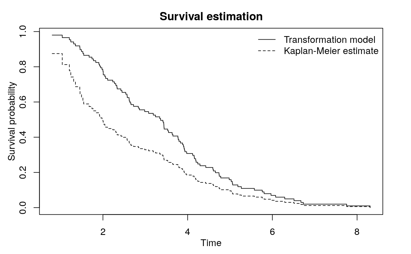
 Transformation parameter by maximizing p-value of the test: -0.3011 

The function trSurvfit gives some important information. The conditional Kendall’s tau for the observed data (before transformation) is 0.5312 with a \(p\)-value < 0.001. The restricted IPW Kendall’s tau (Austin and Betensky, 2014) gives the same result. The transformation parameter, \(a\), turns out to be \(-0.3011\). The estimated survival curve (based on \(a\)) can be plotted with survfit:

> foo <- with(dat, trSurvfit(trun, obs, delta))
> plot(foo)

Simulation

Make a function to call the transformation parameter \(\alpha\).

> do <- function(n){
+   foo <- with(datgen(n), trSurvfit(trun, obs, delta))
+   c(foo$byTau$par[1], foo$byP$par[1])
+ }

Try \(n = 100\) with 100 replicates:

> set.seed(1)
> result <- replicate(100, do(100))

This returns a 2 by 100 matrix. The first row gives \(\hat\alpha\) by maximizing the conditional Kendall’s tau and the second row gives \(\hat\alpha\) by minimizing the \(p\)-value from the conditional Kendall’s tau test.

> summary(t(result))

       V1                V2         
 Min.   :-0.3505   Min.   :-0.3502  
 1st Qu.:-0.3175   1st Qu.:-0.3175  
 Median :-0.2999   Median :-0.2999  
 Mean   :-0.3010   Mean   :-0.3010  
 3rd Qu.:-0.2863   3rd Qu.:-0.2862  
 Max.   :-0.2494   Max.   :-0.2495