Fitting ROC-guided survival tree in rocTree package
Sy Han (Steven) Chiou
2020-01-24
Source:vignettes/rocTree-tree.Rmd
rocTree-tree.RmdIn this vignette, we demonstrate how to use the rocTree function in rocTree package to fit the proposed Receiver Operating Characteristic (ROC) guided survival tree.
Simulated data
We will demonstrate the usage of rocTree function with a simulated data prepared by the simu function.
> library(rocTree)
> set.seed(0)
> dat <- simu(n = 100, cen = 0.25, sce = 2.3, summary = TRUE)
Summary results:
Number of subjects: 100
Number of subjects experienced death: 78
Number of covariates: 2
Time independent covaraites: z1.
Time dependent covaraites: z2.
Number of unique observation times: 100
Median survival time: 0.6822997
> head(dat)
  id        Time death       z1        z2        k        b
1  1 0.002600386     0 1.609865 0.7828513 1.896697 1.604933
2  1 0.004555408     0 1.613574 0.7828513 1.896697 1.604933
3  1 0.020158569     0 1.643168 0.7828513 1.896697 1.604933
4  1 0.027369456     0 1.656845 0.7828513 1.896697 1.604933
5  1 0.047650218     0 1.695311 0.7828513 1.896697 1.604933
6  1 0.053670175     0 1.706729 0.7828513 1.896697 1.604933
The rocTree function
The complete list of arguments in rocTree are as follow:
> args(rocTree)
function (formula, data, id, subset, ensemble = TRUE, splitBy = c("dCON",
    "CON"), control = list())
NULL
The arguments are as follows
-
formulais a formula object, with the response on the left of a~operator, and the predictors on the right. The response must be a survival object returned by the functionSurvfrom thesurvivalpackage. -
datais an optional data frame to interpret the variables occurring in theformula. -
idis an optional vector used to identify the longitudinal observations of subject’s id. The length ofidshould be the same as the total number of observations. Ifidis missing, then each row ofdatarepresents a distinct observation from subjects and all covariates are treated as a baseline covariate. -
subsetis an optional vector specifying a subset of observations to be used in the fitting process. -
ensembleis an optional logical value. IfTRUE(default), ensemble methods will be fitted. Otherwise, the survival tree will be fitted. -
splitByis a character string specifying the splitting algorithm. The available options areCONanddCONcorresponding to the splitting algorithm based on the total concordance measure or the difference in concordance measure, respectively. The default value isdCON. -
controlis a list of control parameters.
The control options
The argument control defaults to a list with the following values:
-
tauis the maximum follow-up time; default value is the 90th percentile of the unique observed survival times. -
maxNodeis the maximum node number allowed to be in the tree; the default value is500. -
numFoldis the number of folds used in the cross-validation. WhennumFold > 0, the survival tree will be pruned; whennumFold = 0, the unpruned survival tree will be presented. The default value is10. -
his the smoothing parameter used in the Kernel; the default value istau / 20. -
minSplitTermis the minimum number of baseline observations in each terminal node; the default value is15. -
minSplitNodeis the minimum number of baseline observations in each splitable node; the default value is30. -
discis a logical vector specifying whether the covariates informulaare discrete (TRUE) or continuous (FALSE). The length ofdiscshould be the same as the number of covariates informula. When not specified, therocTree()function assumes continuous covariates for all. -
Kis the number of time points on which the concordance measure is computed. A less refined time grids (smallerK) generally yields faster speed but a very smallKis not recommended. The default value is 20.
Growing a survival tree
We first load the survival package to enable the Surv() function, which we will use to specify the survival response. The fully grown (un-pruned) time-invariant survival tree can be constructed as follow:
> library(survival)
> system.time(fit <- rocTree(Surv(Time, death) ~ z1 + z2, id = id, data = dat,
+                            ensemble = FALSE, control = list(numFold = 0)))
   user  system elapsed
  0.034   0.000   0.041
The function rocTree returns an object of S3 class with the following major components:
-
Frameis a data frame describe the resulting tree. The columns are -
pindicate which covariate was split at the node. -
leftindicate the row number for the left child (if the current node splittable). -
rightindicate the row number for the right child (if the current node splittable). -
cutValindicate the covariate value (after transformation) being split at the node. -
cutOrdindicate the rank of the covariate value being split at the node. -
ndindicates the node number in display. -
is.terminaldescribe the node characteristic;0if a node is internal,1if a node is a terminal node.
The time-invariant survival tree can be printed directly or with the generic function print.
> fit
 ROC-guided survival tree

 node), split
   * denotes terminal node

Root
 ¦--2) z1 <= 0.52736
 ¦   ¦--4) z2 <= 0.64179
 ¦   ¦   ¦--8) z2 <= 0.29353*
 ¦   ¦   °--9) z2 > 0.29353*
 ¦   °--5) z2 > 0.64179*
 °--3) z1 > 0.52736
     ¦--6) z2 <= 0.67164*
     °--7) z2 > 0.67164*
The survival tree is printed in the structure similar to that in the data.tree package.
Plotting the survival tree
The survival tree can also be plotted with the GraphViz/DiagrammeR engine via the generic function plot.
> plot(fit)plot feature also allows the following arguments adopted from the Graphviz/DiagrammeR environment to be passed to option:
-
typeis an optional character string specifying what to plot. The available options aretreefor plotting survival tree (default),survivalfor plotting the estimated survival probabilities for the terminal nodes, andhazardfor plotting the estimated hazard for the terminal nodes. The following options are available only whentype = tree. -
outputis a string specifying the output type. The possible values aregraphandvisNetwork;graph(the default) renders the graph using thegrVizfunction, andvisNetworkrenders the graph using thevisnetworkfunction. -
digitsthe number of digits to print. -
rankdiris a character string specifying the direction of the tree flow. The available options are top-to-bottom (TB), bottom-to-top (BT), left-to-right (LR), and right-to-left (RL); the default value isTB. -
shapeis a character string specifying the shape style. Some of the available options areellipse,oval,rectangle,square,egg,plaintext,diamond, andtriangle. The default value isellipse. -
nodeOnlyis a logical value indicating whether to display only the node number; the default value isTRUE. -
savePlotis a logical value indicating whether the plot will be saved (exported); the default value isFALSE. -
file_nameis a character string specifying the name of the plot whensavePlot = TRUE. The file name should include its extension. The default value ispic.pdf. -
file_typeis a character string specifying the type of file to be exported. Options for graph files are:png,pdf,svg, andps. The default value ispdf.
The following codes illustrate some of the different options.
> plot(fit, rankdir = "LR", shape = "rect", digits = 2)> plot(fit, shape = "egg", nodeOnly = TRUE)> plot(fit, output = "visNetwork", digits = 2)Pruning the survival tree
Pruning reduces the complexity of the final classifier, and hence improves predictive accuracy by the reduction of overfitting. Setting prune = TRUE in the control list will prune the survival tree. In the following example, we used five-fold cross-validation to choose the tuning parameter in the concordance-complexity measure:
> system.time(fit2 <- rocTree(Surv(Time, death) ~ z1 + z2, id = id, data = dat,
+     ensemble = FALSE, control = list(numFold = 10)))
   user  system elapsed
  0.047   0.000   0.048
> fit2
 ROC-guided survival tree

 node), split
   * denotes terminal node

Root
 ¦--2) z1 <= 0.52736*
 °--3) z1 > 0.52736*
> plot(fit2)fit.
Survival/Hazard estimates at terminal notes
The time-invariant partition considered allows a sparse model and an easy interpretation of the decision rule. At each fixed time \(t\), the tree partitions the survivor population and predicts the instantaneous failure risk. Thus the interpretation at a fixed time point is along the same line as classification and regression trees. Since the risk within each terminal node changes with time, it is essential to look at the hazard curves of each terminal The smoothed hazard estimates at terminal nodes can be easily plotted with the generic function plot with type = "survival" or type = "hazard". The feature is demonstrated below.
> plot(fit2, type = "hazard")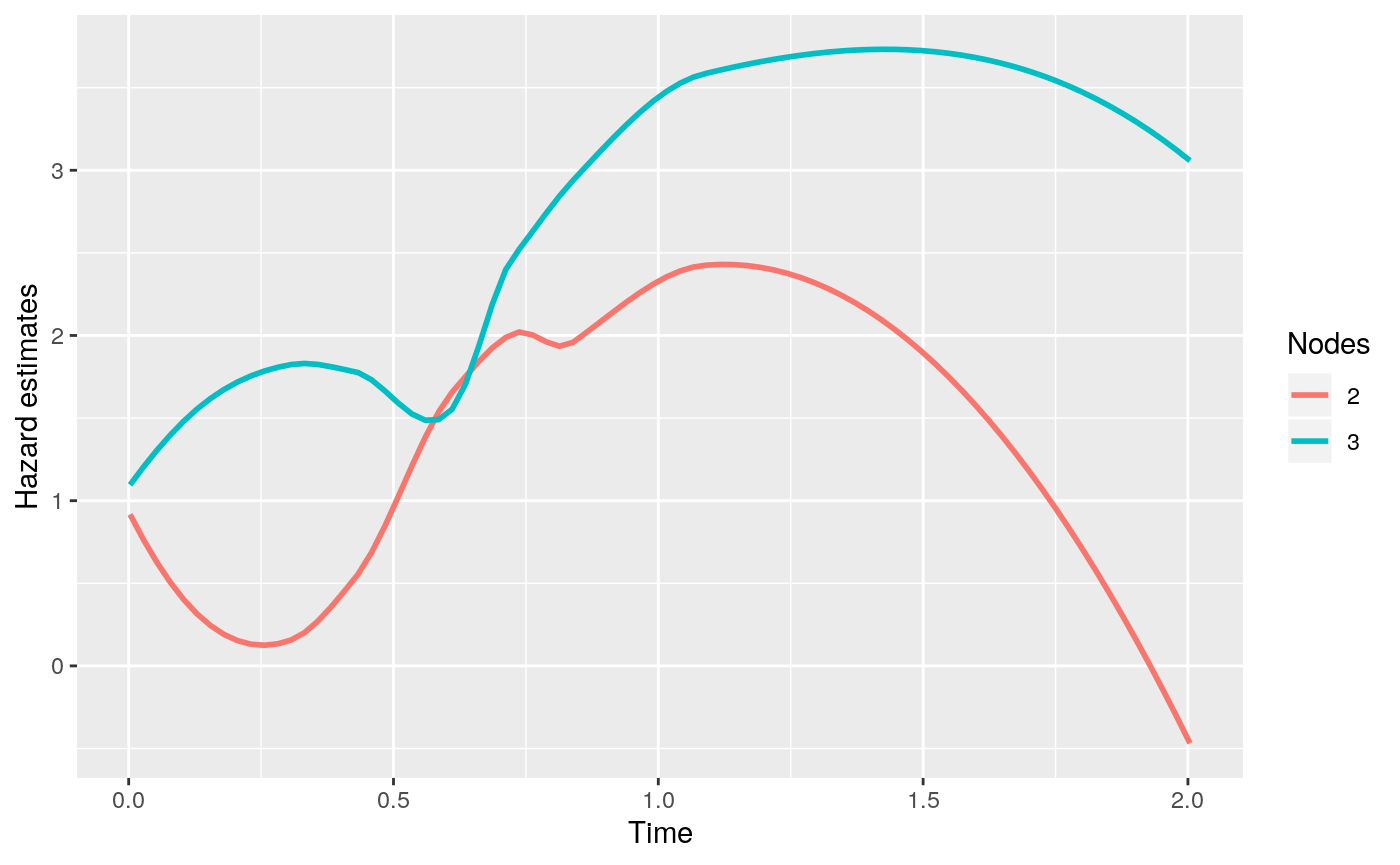
Prediction
Suppose we have a new data that is generated as below:
> newdat <- dplyr::tibble(Time = sort(unique(dat$Time)),
+                         z1 = 1 * (Time < median(Time)),
+                         z2 = 0.5)
> newdat
# A tibble: 100 x 3
      Time    z1    z2
     <dbl> <dbl> <dbl>
 1 0.00260     1   0.5
 2 0.00456     1   0.5
 3 0.0202      1   0.5
 4 0.0274      1   0.5
 5 0.0477      1   0.5
 6 0.0537      1   0.5
 7 0.0564      1   0.5
 8 0.0572      1   0.5
 9 0.0587      1   0.5
10 0.0589      1   0.5
# … with 90 more rows
The predicted survival curve can be plotted with the following codes.
> (pred <- predict(fit2, newdat, type = "survival"))
 Fitted survival probabilities:
         Time Survival
1 0.002600386 0.980953
2 0.004555408 0.980953
3 0.020158569 0.980953
4 0.027369456 0.980953
5 0.047650218 0.980953
> plot(pred)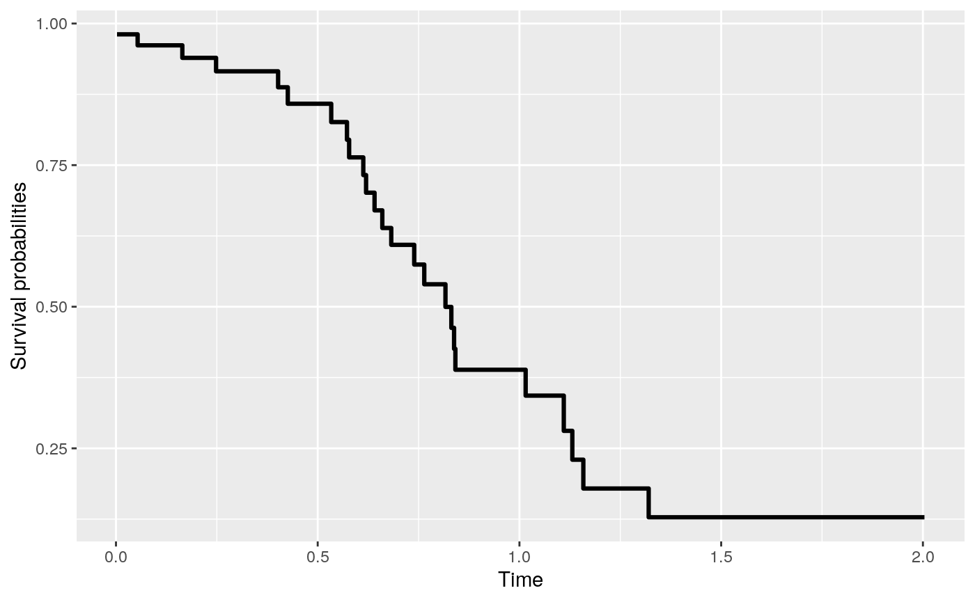
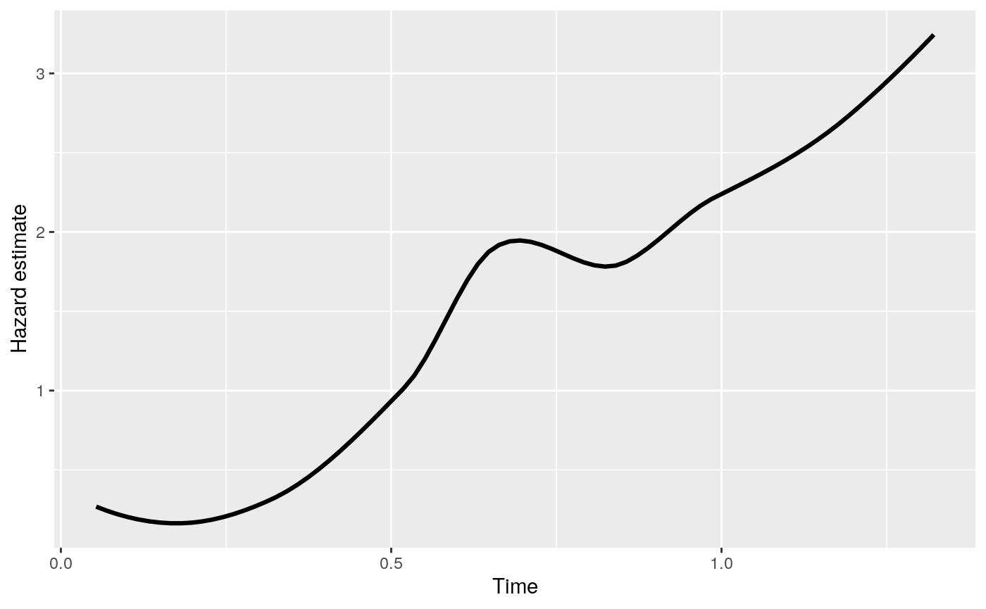
> (pred <- predict(fit2, newdat, type = "hazard"))
 Fitted cumulative hazard:
        Time    hazard
1 0.05336918 0.2931508
2 0.12010736 0.1140868
3 0.18684555 0.2628478
4 0.25358374 0.3424780
5 0.32032193 0.0000000
> plot(pred)